Cifar-10
Cifar-10 Neural Networks
The CIFAR-10 dataset consists of 60000 32x32 colour images in 10 classes, with 6000 images per class. It is then divided into 5 batches with each 10000 images per class and 10000 images for testing.
Get the dataset here
Before reading the code check if you have installed Pytorch . If not consider checking out my guide on it’s installation here.
Download / Clone the code here.
Steps involved in making this neural network :
- Getting the dataset (input)
- Establish the neural network
- Train the neural network
- Validate the neural network
- Plotting graphs
- Test the neural network on test dataset
Getting the dataset :
The dataset is divided into 5 batches for training and validation . One batch is reserved for testing accuracy.
Each image is in rgb format and in a 1-D array form. The first 1024 entries are Red channel , then Green channel and at last Blue channel . The image is of size 32x32 pixels .
We need to transform the data into 3x32x32 dimensions for each image.
The dataset is will look something like this [[3x32x32],[label]].
import pickle
import os
import numpy as np

def unpickle(file):
    import pickle
    with open(file, 'rb') as fo:
        dict = pickle.load(fo, encoding='bytes')
    return dict

def getset(label,data):

	data_set_test = []
	for y,x in zip(label,data):
		X_r = np.reshape(x[:1024],(32,32))
		X_g = np.reshape(x[1024:2048],(32,32))
		X_b = np.reshape(x[2048:],(32,32)) #splitting the rgb elements
		X = np.stack((X_r,X_g,X_b),0)# stacking r , g ,b in 3-d
		data_set_test.append([X,y])
	return data_set_test

#getting raw data from the files
#if you extract cifar10 in your code folder , use the same path
data = []
for i in range(1,6):
	name = "cifar-10-python/cifar-10-batches-py/data_batch_"+ str(i)
	path = os.path.join(name)
	data.append(unpickle(path))

labels_dict = []
for i in data[0] :
	labels_dict.append(i) #getting labels from the dictionary

data_set = []
for i in range(5):
	data_set.append(getset(data[i][labels_dict[1]],data[i][labels_dict[2]]))

'''
print("No of batches",len(data_set))
print("No of pictures in a batch ",len(data_set[0]))
print("data, label",len(data_set[0][0]))
print("Label of first pic",data_set[0][0][1])
print("Data of first pic [r,g,b]",data_set[0][0][0])
'''

training_set =[]
for i in range(len(data_set)):
	for j in range(len(data_set[i])):
		training_set.append(data_set[i][j])

print("No of pictures in training set :",len(training_set))

name = "cifar-10-python/cifar-10-batches-py/test_batch"
path = os.path.join(name)
test = unpickle(path)

test_set = getset(test[labels_dict[1]],test[labels_dict[2]])
print("No of pictures in test set :",len(test_set))

np.save("training_data2.npy",training_set) #saving it

np.save("test_data2.npy",test_set) #saving it
'''
name = "cifar-10-python/cifar-10-batches-py/batches.meta"
path = os.path.join(name)
batch_names = unpickle(path)

print(batch_names)

'''
#^ use the above code to see which label stands for a class
Creating the Neural Network :
I’ve created two neural networks to check which will perform better.
-
Model 1 :
It consists of 2 convolution layers (CNN) and 3 linear layer.
-
Model 2 :
It consists of 3 convolution layers (CNN) and 1 linear layer.
In both models batch norm is used to normalize the data before each convolution layer (CNN) . The first convolution layer will take 3 channels as input because of RGB format.
Packages to import
import os
import cv2
import numpy as np
from tqdm import tqdm
import matplotlib.pyplot as plt
import torch
import torch.nn as nn
import torch.nn.functional as F
import torch.optim as optim
import time
Model 1
class Model(nn.Module):
    def __init__(self):
        super().__init__()
        self.conv1 = nn.Conv2d(3, 8, 5)
        self.pool = nn.MaxPool2d(2, 2)
        self.bn1 = torch.nn.BatchNorm2d(3, eps=1e-05, momentum=0.1, affine=True, track_running_stats=True)
        self.conv2 = nn.Conv2d(8, 16, 5)
        self.bn2 = torch.nn.BatchNorm2d(8, eps=1e-05, momentum=0.1, affine=True, track_running_stats=True)
        self.fc1 = nn.Linear(16 * 5 * 5, 120)
        self.fc2 = nn.Linear(120, 84)
        self.fc3 = nn.Linear(84, 10)

    def forward (self,x):
        x = self.bn1(x)
        x = self.pool(F.relu(self.conv1(x)))
        x = self.bn2(x)
        x = self.pool(F.relu(self.conv2(x)))
        x = x.view(-1, 16 * 5 * 5)
        x = F.relu(self.fc1(x))
        x = F.relu(self.fc2(x))
        x = self.fc3(x)
        return F.softmax(x,dim =1) #using activation function at output to get % or 0-1 values
Model 2
class Model(nn.Module):
    def __init__(self):
        super().__init__()
        self.bn1 = torch.nn.BatchNorm2d(3, eps=1e-05, momentum=0.1, affine=True, track_running_stats=True)
        self.conv1 = nn.Conv2d(3,32,3)
        self.bn2 = torch.nn.BatchNorm2d(32, eps=1e-05, momentum=0.1, affine=True, track_running_stats=True)
        self.conv2 = nn.Conv2d(32,64,3)
        self.bn3 = torch.nn.BatchNorm2d(64, eps=1e-05, momentum=0.1, affine=True, track_running_stats=True)
        self.conv3 = nn.Conv2d(64,128,3)

        x = torch.rand(3,32,32).view(-1,3,32,32)
        self._to_linear = None
        self.convs(x)

        self.fc1 = nn.Linear(self._to_linear,512)
        self.fc2 = nn.Linear(512,10)

    def convs(self,x):
        x = self.bn1(x)
        x = F.max_pool2d(F.relu(self.conv1(x)),(2,2))
        x = self.bn2(x)
        x = F.max_pool2d(F.relu(self.conv2(x)),(2,2))
        x = self.bn3(x)
        x = F.max_pool2d(F.relu(self.conv3(x)),(2,2))
        #print(x.shape)

        if self._to_linear is None:

            self._to_linear = x[0].shape[0]*x[0].shape[1]*x[0].shape[2] # to get the size of 1-d or flattened img

        return x

    def forward (self,x):
        x = self.convs(x)
        x = x.view(-1,self._to_linear)
        x = F.relu(self.fc1(x))
        x = self.fc2(x)
        return F.softmax(x,dim =1) #using activation function at output to get % or 0-1 values
Pre-processing before training :
By pre-processing I mean switching to GPU , seperating training and validation data and initalizing optimizer and loss functions.
model = Model().to(device)
model.double()


training_data = np.load("training_data2.npy",allow_pickle=True) # loading data set

X = torch.Tensor([i[0] for i in training_data])
y = torch.tensor([np.eye(10)[i[1]] for i in training_data])


validation_per = 0.2 # 20%
val_num = int(len(X)*validation_per)
#saving saving 20% of 50000 images for validation

#seperating data sets for training , validating and testing
train_X = X[:-val_num]
train_y = y[:-val_num]

val_X = X[-val_num:]
val_y = y[-val_num:]

#optimization and loss functions

optimizer = optim.Adam(model.parameters() ,lr = 0.001)
loss_function = nn.MSELoss()
Training and validating :
During training the parameters are optimized and loss is reduced . But during validation the parameters are not optimized .
We are also saving the accuracy and loss % of the training data and validation data to plot graph.
def fwd_pass(X,y,train = False):

	X = X.type(torch.DoubleTensor)
	X = X.to(device)
	y = y.to(device)
	#print(X.dtype)
	if train:
		model.zero_grad()
	outputs = model(X)
	check = [torch.argmax(i) == torch.argmax(j) for i,j in zip(outputs,y)]
	acc = check.count(True)/len(check)
	loss = loss_function(outputs,y)

	if train:
		loss.backward()
		optimizer.step()

	return acc,loss

def test(size = 32):
    random_start = np.random.randint(len(val_X)-size)
    X,y = val_X[random_start:random_start+size], val_y[random_start:random_start+size]
    with torch.no_grad():
        val_acc , val_loss = fwd_pass(X, y)
    return val_acc, val_loss

def train():

    batch_size = 100 # no of samples at a time
    epochs = 10 #no of full runs

    with open("model_graph1-10.log","a") as f:
        for epoch in range(epochs):

            for i in tqdm(range(0,len(train_X),batch_size)):

                batch_X = train_X[i:i+batch_size]
                batch_y = train_y[i:i+batch_size]
                acc,loss = fwd_pass(batch_X , batch_y , train= True)

                if i % 50 == 0:
                    val_acc , val_loss = test(size = 100)
                    f.write(f"{MODEL_NAME},{round(time.time(),3)},{round(float(acc),2)},{round(float(loss),4)},{round(float(val_acc),2)},{round(float(val_loss),4)}\n")


MODEL_NAME = f"model -{int (time.time())}"
print(MODEL_NAME)
train()

#saving model

save_path = os.path.join("model1-10.pt")
torch.save(model.state_dict(),save_path)
Plotting graphs :
The graph is used to check if the model is worth training or not.
Two graphs are plotted :
- Training accuracy and validation accuracy vs time
- Training loss and validation loss vs time
import matplotlib.pyplot as plt
from matplotlib import style
style.use("ggplot")
model_name = "model -1590133058" # model name (check inside the log folder)
def create_acc_loss_graph(model_name):
#graph values
contents = open("model_graph1-10.log","r").read().split('\n')
times = []
accuracies = []
losses = []
val_accs = []
val_losses = []
for c in contents:
if model_name in c:
name , timestamp , acc , loss , val_acc , val_loss = c.split(",")
times.append(float(timestamp))
accuracies.append(float(acc))
losses.append(float(loss))
val_accs.append(float(val_acc))
val_losses.append(float(val_loss))
fig = plt.figure()
ax1 = plt.subplot2grid((2,1), (0,0))
ax2 = plt.subplot2grid((2,1), (1,0), sharex=ax1)
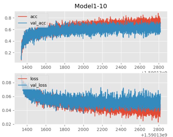
ax1.set_title("Model1-10") # title name
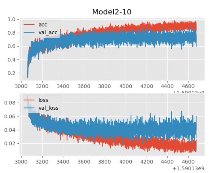
ax1.plot(times, accuracies, label="acc")
ax1.plot(times, val_accs, label="val_acc")
ax1.legend(loc=2)
ax2.plot(times,losses, label="loss")
ax2.plot(times,val_losses, label="val_loss")
ax2.legend(loc=2)
plt.show()
create_acc_loss_graph(model_name)
Model 1
Model 2
Testing the Neural Network :
The test dataset is used to check the accuracy of the neural network.
Now to test the neural network , copy paste the model you want to test from above and use the code below.
model = Model()
save_path = os.path.join("model2-10.pt")
model.load_state_dict(torch.load(save_path))
model.eval()
model.double()
test_data = np.load("test_data2.npy",allow_pickle=True) # loading data set
test_X = torch.tensor([i[0] for i in test_data])
test_y = torch.tensor([np.eye(10)[i[1]] for i in test_data])
#print(test_X[0])
batch_size = 100
acc = 0
label = { "aeroplane":0,"automobile":0,"bird":0,"cat":0,"deer":0,
"dog":0,"frog":0,"horse":0,"ship":0,"truck":0 }
for i in tqdm(range(0,len(test_X),batch_size)):
batch_X = test_X[i:i+batch_size].view(-1,3,32,32)
batch_y = test_y[i:i+batch_size]
batch_X = batch_X.type(torch.DoubleTensor)
output = model(batch_X)
for i,j in zip(output,batch_y):
x = torch.argmax(i)
y = torch.argmax(j)
if x == y :
acc += 1
if y == 0:
label["aeroplane"] += 1
elif y == 1:
label["automobile"] += 1
elif y == 2:
label["bird"] += 1
elif y == 3:
label["cat"] += 1
elif y == 4:
label["deer"] += 1
elif y == 5:
label["dog"] += 1
elif y == 6:
label["frog"] += 1
elif y == 7:
label["horse"] += 1
elif y == 8:
label["ship"] += 1
elif y == 9:
label["truck"] += 1
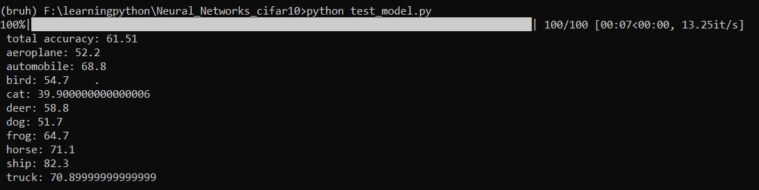
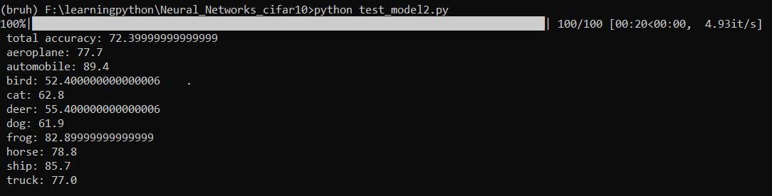
total_accuracy = acc/len(test_X) *100
print("Total accuracy : ",total_accuracy)
#Getting accuracy of each element
for i in label:
label[i] = label[i]/1000 *100
print(f" {i} : {label[i]} ")
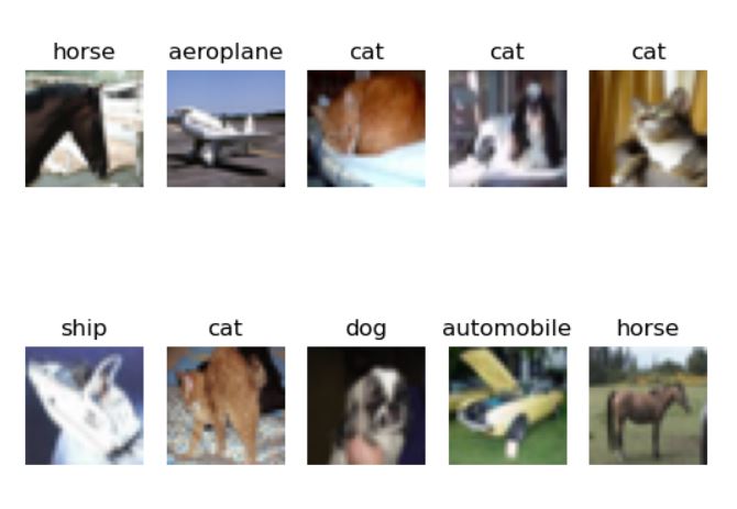
#checking for last 10 images
pic = test_X[-10:]
prediction = output[-10:]
titles = { 0:"aeroplane",1:"automobile",2:"bird",3:"cat",4:"deer",
5:"dog",6:"frog",7:"horse",8:"ship",9:"truck" }
c = 1
for i in range(10):
x = pic[i].numpy() #plotting the images
y = torch.argmax(prediction[i]).tolist()
image = cv2.merge((x[2],x[1],x[0]))
plt.subplot(2,5,c)
plt.axis("off")
plt.title(titles[y])
plt.imshow(cv2.cvtColor(image, cv2.COLOR_BGR2RGB))
c += 1
plt.show()
Inference :
Output of Model 1 after training for 10 epochs
Output of Model 2 after training for 10 epochs
Prediction of last 10 images of test dataset