Cats vs Dogs
Cats vs Dogs - Neural Networks
I’ve created a neural network with 4 hidden layers which take 1 channel input and give 2 outputs (Cat / Dog). (Used convolution for 3 hidden layers and linear for 1 hidden layer)
Before reading the code check if you have installed Pytorch . If not consider checking out my guide on it’s installation here.
Download / Clone the code here.
Steps involved in making this neural network :
- Getting the dataset (input)
- Establish the neural network
- Train the neural network
- Testing the neural network
- Plotting graphs
- Test the neural network on images outside dataset
Packages to be imported
import os
import cv2
import numpy as np
from tqdm import tqdm
import matplotlib.pyplot as plt
import torch
import torch.nn as nn
import torch.nn.functional as F
import torch.optim as optim
import time
Activating the GPU :
if torch.cuda.is_available():
    device = torch.device("cuda:0")
    print("running on the GPU")

else:
    device = torch.device("cpu")
    print("running on the CPU")

# If gpu is avaliable it will do calculations on the GPU
Getting the dataset :
I’ve used the dataset from microsoft . Download Extract the folder “PetImages” to your code folder.
Now , you need to convert the images in those folder to an array. In this code I’ve converted the image to grayscale and resized it to 50x50 pixels. Then used np.array to convert the image to a matrix.
#make sure to extract kaggle PetTmages folder in the same file as your code

REBUILD_DATA = True # True - to build a dataset , false - to not build a dataset

class DogsVSCats():
    IMG_SIZE = 50 # making the img 50x50 pixels
    CATS = "PetImages/Cat"
    DOGS = "PetImages/Dog"
    LABELS = {CATS: 0, DOGS: 1}
    training_data = []
    catcount = 0
    dogcount = 0

    def make_training_data(self):
        for label in self.LABELS:
            for f in tqdm(os.listdir(label)): #runs till the last img in the directory
                if "jpg" in f: #getting only jpg
                    try: #used for error handling because there are some corrupt imgs
                        path = os.path.join(label, f)
                        img = cv2.imread(path, cv2.IMREAD_GRAYSCALE)#converting to gray scale to reduce complexity
                        img = cv2.resize(img, (self.IMG_SIZE, self.IMG_SIZE))
                        # converts the img to 50x50 px
                        self.training_data.append([np.array(img), np.eye(2)[self.LABELS[label]]])
                        # assigns [1,0] as cat and [0,1] as dog (using one hot vector)

                        if label == self.CATS: #used to check balance of inputs b/w cats and dogs
                            self.catcount += 1
                        elif label == self.DOGS:
                            self.dogcount += 1
                    except Exception as e:
                        pass

        np.random.shuffle(self.training_data) #shuffling the cats and dogs data for efficient generalization
        np.save("training_data.npy",self.training_data) #saving it
        print("Cats :",self.catcount) #checking the count
        print("Dogs :",self.dogcount)

if REBUILD_DATA: #To build the data REBUILD_DATA = True
    dogsvcats = DogsVSCats()
    dogsvcats.make_training_data()
The data given should be balanced . Imagine in this case we got two types of inputs cats and dogs , So the data should contain 50% of cat images and 50% of dog images .
Try avoiding data that is not balanced . It would cause the neural network to memorize than generalize. After creating the data set you can either delete the code or change REBUILD_DATA = False on the top.
Creating the neural network :
This neural network contains 4 hidden layers , 3 2-d convolution layers and 1 linear layer .
The first layer gets input from 1 channel and has 32 neurons. The second layer gets input from first layer and has 64 neurons. The third layer gets input from second layer and has 128 neurons.
To pass data from the convolution layer to the linear layer , we need to flatten the image. So I’ve created a random matrix of 50x50 size to find the shape of data after it passes the convolution layer. The linear layer has 512 neurons and gives the output as a probability of Cats vs Dogs.
Activation function used : Rectified Linear
Activation function used on output : softmax
class Net(nn.Module):
    def __init__(self):
        super().__init__() #creating hidden layers
        #no of channels used is 1
        # 3 hidden layers with 32 / 64 / 128 neurons . this caculates in convolution 2d
        self.conv1 = nn.Conv2d(1,32,5) # 1 channel , 32 neurons , 5 - kernel size
        self.conv2 = nn.Conv2d(32,64,5)
        self.conv3 = nn.Conv2d(64,128,5)

        x = torch.randn(50,50).view(-1,1,50,50) # we need to convert 2d to 1d so we need to find the 1d size
        self._to_linear = None # using random generated data to find the size
        self.convs(x)

        self.fc1 = nn.Linear(self._to_linear,512) # hidden layer with 512 neurons
        self.fc2 = nn.Linear(512,2) # out put 2 neurons cat / dog

    def convs(self,x):
        x = F.max_pool2d(F.relu(self.conv1(x)),(2,2))#using pooling and activation function to round off values
        x = F.max_pool2d(F.relu(self.conv2(x)),(2,2))
        x = F.max_pool2d(F.relu(self.conv3(x)),(2,2))

        #print(x[0].shape)

        if self._to_linear is None:

            self._to_linear = x[0].shape[0]*x[0].shape[1]*x[0].shape[2] # to get the size of 1-d or flattened img

        return x

    def forward (self,x): #used to pass through the hidden layers
        x = self.convs(x) # calculating convolution first
        x = x.view(-1,self._to_linear) # converting to linear
        x = F.relu(self.fc1(x)) # calculating linear
        x = self.fc2(x) # getting output
        return F.softmax(x,dim =1) #using activation function at output to get % or 0-1 values
Training the neural network :
Before training the network, you need to convert the np.array to a tensor. Then you need to seperate a part of the images to train and a part of the images to test the neural network. These two sets of images should not overlap.
Coverting to tensor
X = torch.Tensor([i[0] for i in training_data]).view(-1,50,50)
#converting numpy array to tensor
X = X/255.0
# since gray scale is of pixels from 0-255 converting to 0-1
y = torch.Tensor([i[1] for i in training_data])
#Getting the labels for corresponding image values
VAL_PCT = 0.1  # lets reserve 10% of images for validation (test images)
val_size = int(len(X)*VAL_PCT)
#print(val_size)

train_X = X[:-val_size] #gets all images other than test images
train_y = y[:-val_size]

test_X = X[-val_size:] #gets all test images
test_y = y[-val_size:]
You want to add an optimizer and loss function , so that the optimizer can tune the parameters to reduce loss.
optimizer = optim.Adam(net.parameters(), lr=0.001)
#using optimizer to tune parameters and learning rate 0.001
loss_function = nn.MSELoss()
#using mean square error to calculate loss ( because one hot vector)
Before training the neural network . The test and train function are both going to calculate loss and accuracy only difference is in train function has to optimize and reduce loss . So we create a funtion which can do that and just call them in train / test function.
def fwd_pass(X, y, train=False):
    if train:
        net.zero_grad()#makes gradient zero
    outputs = net(X)
    matches  = [torch.argmax(i)==torch.argmax(j) for i, j in zip(outputs, y)]
    #To check if the ouput matches the labels
    acc = matches.count(True)/len(matches)
    loss = loss_function(outputs, y)
    #calculating accuracy and loss %
    if train:
        loss.backward()
        optimizer.step()
        #reducing loss and increasing accuracy
Train function :
In this function , we are going to pass the train_X in net()/model to get the output.
The BATCH_SIZE value can be varied according to your GPU capabilities.
EPOCHS is how many time you want to train the network.
For this model EPOCHS around 5-10 will give accuracy around 80% . But after that it does not improve graph will be shown below.
def train():
    BATCH_SIZE = 100 #no of samples in a go
    EPOCHS = 8 # no of full passes
    with open("model_graph.log","a") as f: #to register acc,loss of test and train images for plotting graph
        for epoch in range(EPOCHS):

            for i in tqdm(range(0,len(train_X),BATCH_SIZE)): #there are around 25500(approx) images
                #so the loop runs for 25500/100 times that is 255 times
                batch_X = train_X[i:i+BATCH_SIZE].view(-1,1,50,50).to(device)
                batch_y = train_y[i:i+BATCH_SIZE].to(device)
                acc,loss = fwd_pass(batch_X , batch_y , train= True)
                #getting acc and loss of train images
                if i % 50 == 0: #updating loss and acc after every 50 iterations
                    val_acc , val_loss = test(size = 100) #getting acc and loss of test images after training 50 times
                    f.write(f"{MODEL_NAME},{round(time.time(),3)},{round(float(acc),2)},{round(float(loss),4)},{round(float(val_acc),2)},{round(float(val_loss),4)}\n")

train()
#model name will be used to calculate the graph , take note of it in the output window
MODEL_NAME = f"model -{int (time.time())}"
print(MODEL_NAME)
#giving our model a name
Testing the neural network :
Testing the neural network gives you a good idea on how the neural network will behave on images outside the dataset. It is usually used to validate the network and optimize it further but, I’ve not done it because it is my first project on neural networks.
In my case I’ve used test to calculate the acc and loss on test_X images .
#To test if the neural network is trained correctly by using the images validated
def test(size = 32):
    random_start = np.random.randint(len(test_X)-size) #getting a random slice of given size
    X,y = test_X[random_start:random_start+size], test_y[random_start:random_start+size]
    with torch.no_grad(): #calculating acc and loss for the test images
        val_acc , val_loss = fwd_pass(X.view(-1, 1,50,50).to(device) , y.to(device))
    return val_acc, val_loss
Plotting the graph :
To visualize if your neural network is improving , Plot two graphs accuracy vs time and loss vs time .
You need to plot accuracy / loss of train_X and test_X in the same Y- axis.
The time stamp is same for all graphs.
Run this in a separate file.
import matplotlib.pyplot as plt
from matplotlib import style


style.use("ggplot")

model_name = "model -1589867511"
#copy the model name paste it here , from previous program or just copy the model number from model_graph.log

def create_acc_loss_graph(model_name):
	contents = open("model_graph.log","r").read().split('\n')

	times = []
	accuracies = []
	losses = []

	val_accs = []
	val_losses = []

	for c in contents:
		if model_name in c:
			name , timestamp , acc , loss , val_acc , val_loss = c.split(",")

			times.append(float(timestamp))
			accuracies.append(float(acc))
			losses.append(float(loss))

			val_accs.append(float(val_acc))
			val_losses.append(float(val_loss))
#getting values of time , accuracy and loss in a list
	fig = plt.figure()

	ax1 = plt.subplot2grid((2,1), (0,0))
	ax2 = plt.subplot2grid((2,1), (1,0), sharex=ax1)
#plotting two graphs accuracy vs time and loss vs time

	ax1.plot(times, accuracies, label="acc")
	ax1.plot(times, val_accs, label="val_acc")
	ax1.legend(loc=2)
	ax2.plot(times,losses, label="loss")
	ax2.plot(times,val_losses, label="val_loss")
	ax2.legend(loc=2)
	plt.show()

create_acc_loss_graph(model_name)
The graph after 30 EPOCHS
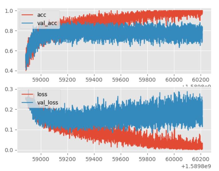
You can see the deviation between train_X and test_X . It means that train_X just memorized all the images in dataset and thats why the accuracy/loss of test_X does not increase/decrease.
It would be enough to train it for 5-10 EPOCHS.
The graph after 8 EPOCHS
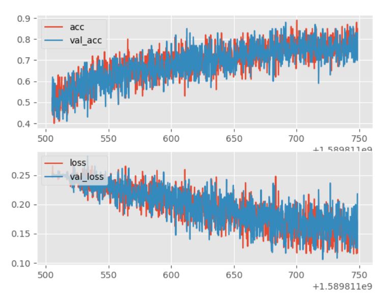
You can see that the accuracy is around 80%-70% . Which is the maximum for this model , training further would be useless.
It could be improved by validating , which maybe included in the future.
Checking outside the dataset :
First you need to save the parameters of your model , then you don’t have to train every single time.
save_path = os.path.join("model.pt")
torch.save(net.state_dict(),save_path) #type this in the main program to save
#saving parameters
Then to test it , create an another file . Copy paste the model only and load the parameters of your model.
This is my code to just check if the image has a dog / cat.
import os
import cv2
import numpy as np
from tqdm import tqdm
import matplotlib.pyplot as plt
import torch
import torch.nn as nn
import torch.nn.functional as F
import torch.optim as optim
import time

# you need to initalize the class again
class Net(nn.Module):
    def __init__(self):
        super().__init__()
        # 3 hidden layers with 32 / 64 / 128 neurons . this caculates in convolution 2d
        self.conv1 = nn.Conv2d(1,32,5) # 1 input , 32 neurons , 5 - kernel size
        self.conv2 = nn.Conv2d(32,64,5)
        self.conv3 = nn.Conv2d(64,128,5)

        x = torch.randn(50,50).view(-1,1,50,50) # we need to convert 2d to 1d so we need to find the 1d size
        self._to_linear = None # using random generated data to find the size
        self.convs(x)

        self.fc1 = nn.Linear(self._to_linear,512) # calculation in 1-d using 512 neurons
        self.fc2 = nn.Linear(512,2) # out put 2 neurons cat / dog

    def convs(self,x):
        x = F.max_pool2d(F.relu(self.conv1(x)),(2,2))#using pooling and activation function to round off values
        x = F.max_pool2d(F.relu(self.conv2(x)),(2,2))
        x = F.max_pool2d(F.relu(self.conv3(x)),(2,2))

        #print(x[0].shape)

        if self._to_linear is None:

            self._to_linear = x[0].shape[0]*x[0].shape[1]*x[0].shape[2] # to get the size of 1-d or flattened img

        return x

    def forward (self,x):
        x = self.convs(x) # calculating convolution first
        x = x.view(-1,self._to_linear) # converting to linear
        x = F.relu(self.fc1(x)) # calculating linear
        x = self.fc2(x) # getting output
        return F.softmax(x,dim =1) #using activation function at output to get % or 0-1 values

net = Net()
#loading the saved parameters
save_path = os.path.join("model.pt")
net.load_state_dict(torch.load(save_path))
net.eval()

# To check if a random image is a dog or a cat
while True:

    get_path = input("Enter the path of the image :")

    #save_path = os.path.join("Enter image name")
    #if the image is in ur code folder use the above code

    img = cv2.imread(get_path)

    X = cv2.cvtColor(img, cv2.COLOR_BGR2GRAY)
    X = cv2.resize(X, (50,50))

    X = torch.Tensor(np.array(X)).view(-1,50,50)
    #gets all the image values from dataset , in the size 50x50
    X = X/255.0
    # since gray scale is of pixels from 0-255 converting to 0-1

    cod = net((X.view(-1,1,50,50)))
    check_cod = torch.argmax(cod)
    print(cod,check_cod)
    if check_cod == 0:
        animal = "Cat"

    else :
        animal = "Dog"

    plt.axis("off")
    plt.title(animal)
    plt.imshow(cv2.cvtColor(img, cv2.COLOR_BGR2RGB))
    plt.show()

    yorn = input("Do you want to check for another image (y/n) ?")

    if yorn == "n" or yorn == "N" :
        break
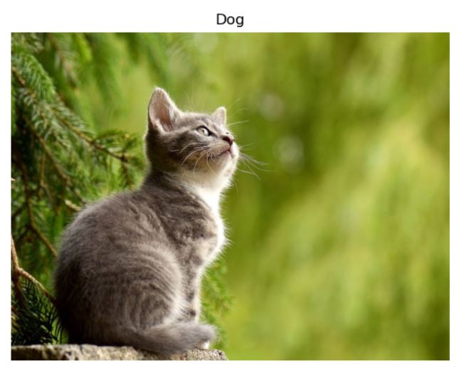
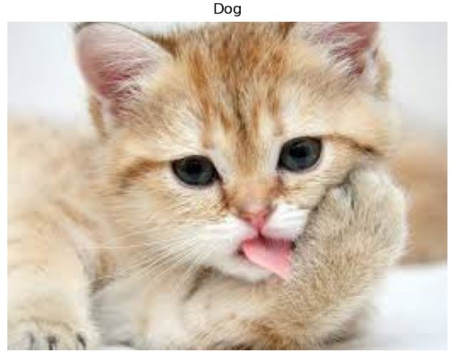
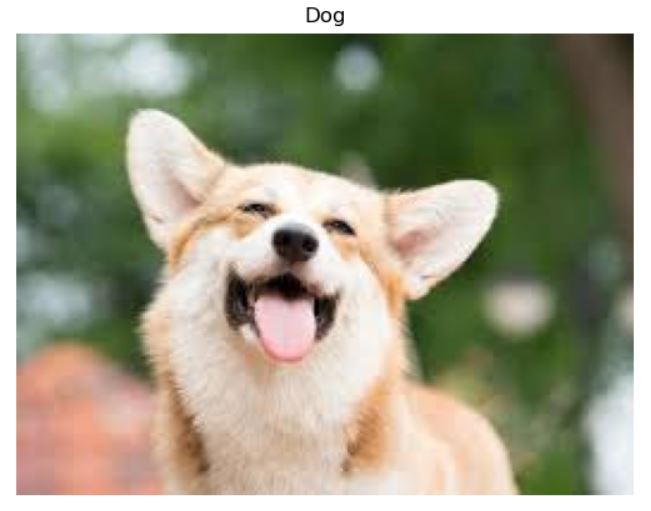
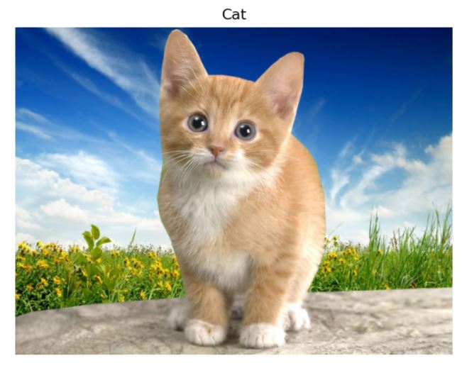
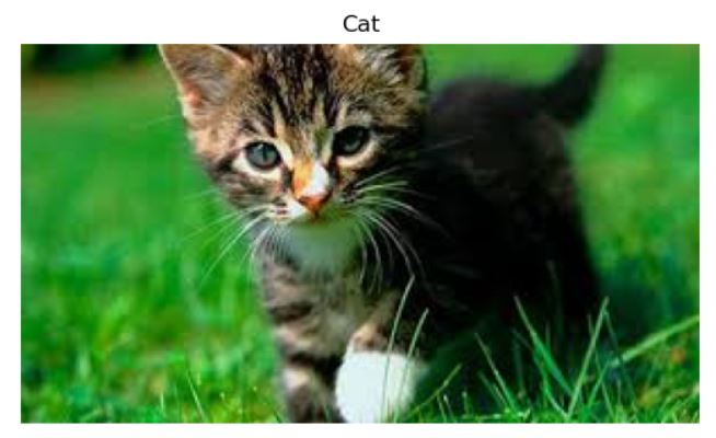
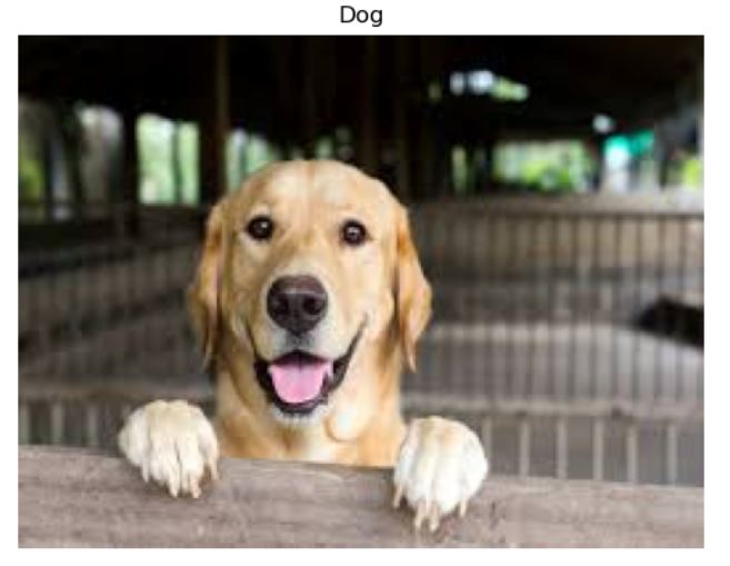
I downloaded 6 images and ran them through this code to check the output .
I got 4 out of 6 correct .
Correct outputs :
Wrong outputs :